Understanding the Lognormal Distribution
April 25, 2026
If one is very fortunate enough not to use Twitter, one will be able to avoid interacting with a lot of terrible people, especially racists or sexists individuals. (I still refer to the platform as Twitter) People who are obsessed with immutable characteristics are also obsessed with bell curves and distributions. However, this obsession has done little to improve their conceptual understanding of one of the most fundamental concepts in probability and statistics.
If one values their sanity, I do not recommend spending a significant amount of time on Twitter. However, it will not take very long to find someone using their statistical illiteracy to justify any abhorrent opinion. Such is the case with Mr WearyWendigo, who (upon clicking on the post and reading the thread) seems to be very confused about distributions, normal distributions, standard normal distributions and many other distributions.
It should be obvious that a lognormal distribution is not a normal distribution. Let $X$ be a normal random variable with mean $\mu$ and variance $\sigma^2$, we have the following:
\[\begin{equation} X\sim\mathcal{N}(\mu,\sigma^2) \end{equation}\]If we define random variable $Y$ as
\[\begin{equation} Y=\exp(X) \end{equation}\]We say that $Y$ is lognormally distributed with parameters $\mu$ and $\sigma$ or
\[\begin{equation} \log Y\sim\mathcal{N}(\mu,\sigma^2), \end{equation}\]which means that the logarithm of the variable is normally distributed, not the “range of the artefacts,” or whatever that means. So if the random variable $Y$ refers to height, then height is lognormal, and the $\log Y$ would form a bell curve.
Non-negativity
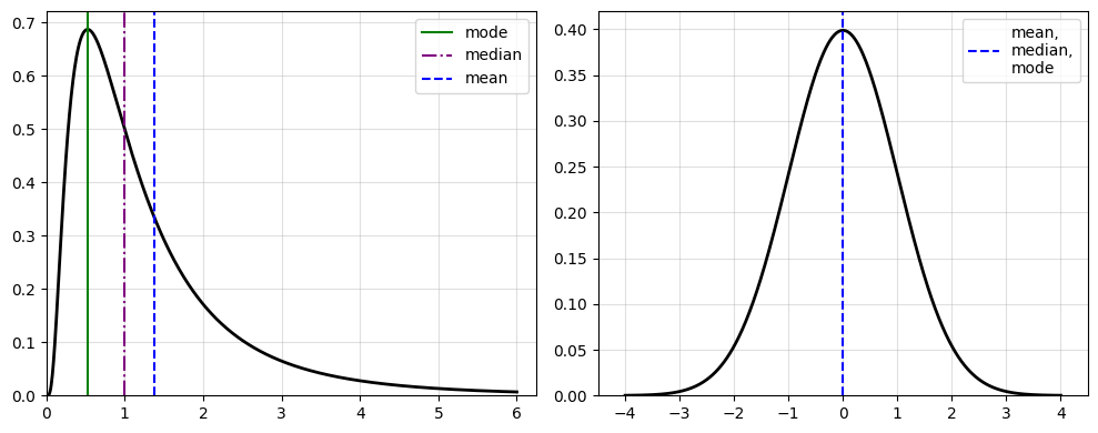
One of the most obvious things to observe is that $Y$ is a non-negative random variable (Figure $1$), since $e^x$ is positive for any value of $x$. Therefore, the lognormal distribution is often used in cases where non-negativity is an important property of the data being modelled.
Moments
The parameters $\mu$ and $\sigma^2$ are the mean and variance of $X$. However, they are not the mean and variance of $Y$. Therefore, the lognormal cannot be a “skewed standard,” as Mr. WearyWendigo suggested. So the mean of $Y$ is denoted by the following
\[\begin{equation} \mathbb{E}[Y]=\mathbb{E}\left[\exp(X)\right]=\exp \left\lbrace\mu+\frac{1}{2}\sigma^2\right\rbrace \end{equation}\]We want the $k$-th moment $Y=e^{X}$ when $X\sim\mathcal(\mu,\sigma^2)$, so we want to simplify the following:
\[\begin{equation} \begin{aligned} \mathbb{E}\left[Y^k\right]&=\mathbb{E}\left[e^{Xk}\right]\\ &=\int_{-\infty}^{\infty}e^{xk}\frac{1}{\sqrt{2\pi\sigma^2}}e^{-\frac{1}{2}\left(\frac{x-\mu}{\sigma}\right)^2}dx\\ &=\int_{-\infty}^{\infty}\frac{1}{\sqrt{2\pi\sigma^2}}e^{-\frac{1}{2}\left(\frac{x-\mu}{\sigma}\right)^2+xk} dx\\ &=\int_{-\infty}^{\infty}\frac{1}{\sqrt{2\pi\sigma^2}}e^{-\frac{1}{2\sigma^2}(x-\mu)^2+2\sigma^2xk}dx\\ &=\int_{-\infty}^{\infty}\frac{1}{\sqrt{2\pi\sigma^2}}e^{-\frac{1}{2\sigma^2}\left(x^2-\mu^2-2\sigma\mu-2\sigma^2xk\right)}dx\\ &=\int_{-\infty}^{\infty}\frac{1}{\sqrt{2\pi\sigma^2}}e^{-\frac{1}{2\sigma^2}\left[\left(x^2-\mu^2-2\sigma\mu-2\sigma^2xk\right)+\overbrace{\left(2\sigma^2k\mu+k^2\sigma^4\right)-\left(2\sigma^2k\mu+k^2\sigma^4\right)}^{\text{Adding Zero}}\right]}dx\\ &=\int_{-\infty}^{\infty}\frac{1}{\sqrt{2\pi\sigma^2}}e^{-\frac{1}{2\sigma^2}\left[\left(x-\mu-k\sigma^2\right)^2-\left(2\sigma^2k\mu+k^2\sigma^4\right)\right]}dx\\ &=\int_{-\infty}^{\infty}\frac{1}{\sqrt{2\pi\sigma^2}}e^{-\frac{1}{2\sigma^2}\left(x-\mu-k\sigma^2\right)^2+\frac{1}{2\sigma^2}\left(\cancel{2\sigma^2}k\mu+k^2\sigma^{\cancel{4}^2}\right)}dx\\ &=e^{k\mu+\frac{1}{2}k^2\sigma^2}\int_{-\infty}^{\infty}\frac{1}{\sqrt{2\pi\sigma^2}}e^{-\frac{1}{2\sigma^2}\left(x-\mu-k\sigma^2\right)^2}dx\\ &=e^{k\mu+\frac{1}{2}k^2\sigma^2}\cdot 1\\ \end{aligned} \end{equation}\]Since the integral will evaluate to $1$, we have the following
\[\begin{equation} \mathbb{E}\left[e^{Xk}\right]=\exp \left\lbrace k\mu+\frac{1}{2}k^2\sigma^2\right\rbrace . \end{equation}\]The variance is fairly easy to evaluate by way of Equation $6$. Since we already know the expectation of $Y$, we have the following
\[\begin{equation} \begin{aligned} \text{Var}(Y)&=\mathbb{E}\left[Y^2\right]-\mathbb{E}[Y]^2\\ &=e^{2\mu+\frac{1}{2}\cdot 4\sigma^2}-\left[e^{\mu+\frac{1}{2}\sigma^2}\right]^2\\ &=e^{2\mu+2\sigma^2}-e^{2\mu+\sigma^2}\\ \end{aligned} \end{equation}\]By factoring exponents, we have the following for the variance,
\[\begin{equation} \text{Var}(Y)=\left(\exp\left\lbrace \sigma^2\right\rbrace-1\right)\exp \left\lbrace2\mu+\sigma^2\right\rbrace. \end{equation}\]Cumulative Density Function
The cumulative density function (CDF) of $Y$ is
\[\begin{equation} F_Y(y)=\Phi \left(\frac{\log y-\mu}{\sigma}\right), \end{equation}\]where $\Phi(x)$ is CDF of the standard normal distribution, which denotes the following
\[\begin{equation} \mathbb{P}(Y\leq y)=\mathbb{P}(X\leq\log y) \end{equation}\]Using Equation $9$, we can derive the probability density function (PDF) of $Y$ by differentiating the CDF of $Y$. If we let $\Phi(x)$ and $\varphi(x)$ denote the CDF and PDF of $X$ respectively. Then the PDF of $Y$ is the following:
\[\begin{equation} \begin{aligned} f_Y(y)&=\frac{d}{dy}\mathbb{P}(Y\leq y)\\ &=\frac{d}{dy}\mathbb{P}(X\leq\log y)\\ &=\frac{d}{dy}\Phi\left(\frac{\log y-\mu}{\sigma}\right)\\ &=\varphi\left(\frac{\log y-\mu}{\sigma}\right)\frac{d}{dy}\left(\frac{\log y-\mu}{\sigma}\right)\\ &=\varphi\left(\frac{\log y-\mu}{\sigma}\right)\frac{1}{\sigma}\frac{d}{dy}\left(\log y-\mu\right)\\ &=\varphi\left(\frac{\log y-\mu}{\sigma}\right)\frac{1}{\sigma}\cdot\frac{1}{y}\\ &=\varphi\left(\frac{\log y-\mu}{\sigma}\right)\frac{1}{y\sigma}\\ \end{aligned} \end{equation}\]Therefore, using the definition of $\varphi(x)$, we have the following
\[\begin{equation} f_Y(y)=\frac{1}{y\sigma\sqrt{2\pi}}\exp\left\lbrace-\frac{1}{2}\left[\frac{\log y-\mu}{\sigma}\right]^2\right\rbrace \end{equation}\]Central Tendency
From Equation $8$, we can use the CDF to compute the median of $Y$, denoted by
\[\begin{equation} m:=\exp(\mu) \end{equation}\]and use the PDF to compute the mode, denote by
\[\begin{equation} d:=\exp(\mu-\sigma^2). \end{equation}\]The proof for the mode is very tedious and very long, so you readers can review the Book of Statistical Proofs. So under a lognormal distribution, we can see from Equation $6,13,14$ that the following should hold
\[\begin{equation} \exp(\mu-\sigma^2)\leq\exp(\mu)\leq\exp\left(\mu+\frac{1}{2}\sigma^2\right). \end{equation}\]Common areas were we see lognormal distributions include income, wealth, stock returns, biology, etc. Very important distinction between a normal, or even a standard normal distribution. Then again, we are reviewing probability theory, which has some elements of multivariable calculus. It would be safe if bigots were capable of understanding these things, they would not be bigots.