Principal Component Analysis

November 02, 2025

Principal component analysis (PCA) (Pearson, 1901; Hotelling, 1933) is a workhorse in statistics. It is often the first tool we reach for when performing exploratory data analysis or dimension reduction. The method is simple, fast, and theoretically well-understood, and it is the bedrock upon which many more complex dimension-reduction methods are built.

The goal of this post is to understand PCA in detail. We will start by visualizing the big idea, exploring the key concepts with as little mathematical detail or jargon as needed. In the next two sections, we will formalize our intuitions from the first section and then derive some basic properties of PCA. Finally, we will conclude with a complete PCA implementation to reproduce a famous result: eigenfaces (Turk & Pentland, 1991).

1. Visualizing the big idea

Imagine we are naturalists visiting a strange new island, tasked with naming, defining, and classifying the birds we find there. We plan to do this by first observing and cataloguing as many birds as possible and then grouping them based on their shared characteristics. However, how do we decide when to place a bird into a given group?

For example, compare the ramphastos (Figure 1, bottom left) to the rufous-collared kingfisher (Figure 1, top right). We may think that these two birds are obviously different species, but why do we think that? The answer is that these two birds are more similar to many other birds than they are to each other. We can easily find two groupings of birds, say of toucans and kingfishers, such that the variation between the two groups is larger than the variation within each group.

How can we make this idea of intra-versus extra-group variation more precise? One idea would be to record many features of each bird we see: coloring, size, location, plumage, beak shape, and so forth. Then we could look for features along which all the birds on this island had the most variation. We could use this variance-maximizing feature to help us split birds into meaningful groups.

It is worth asking whether features with lots of variation are useful for our task, so consider the opposite: imagine that all the birds on the island had a particular feature with almost no variation. Suppose, for example, that all the birds were white. This feature, coloring, would be almost useless for the classification of the islands’ birds. However, the fact that all the birds on the island are white does not mean that all the birds belong to the group. If some white birds have large, hooked beaks while others have short, stout beaks, we might wonder whether this beak shape is important for our task. This is the basic logic behind looking for features with lots of variation.

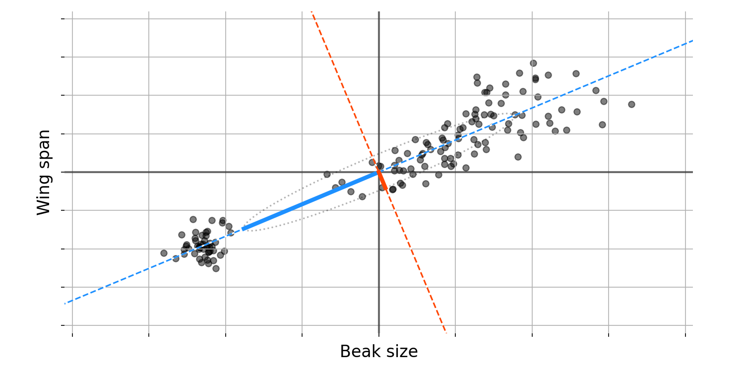
Let us try to visualise this idea with some data. Imagine we plot two bird features against each other, say beak size against (Figure 1). After plotting these data, we notice something: since these two features are correlated, the axis along which variation between birds is maximised is neither just beak size nor just wing span. Instead, the axis along which variation is maximised is some combination of both features, as represented by the blue dashed line. This diagonal line can be thought of as representing a new, composite feature or dimension. We cannot precisely interpret this composite feature, but we might hypothesize that it represents “bird size”.

In the language of statistics and linear algebra, we call the direction of this blue dashed line the first principal component (PC). More formally, the first PC is a unit vector that defines an axis along which the variance of our data is maximised.

After finding this first PC, what can we do? We might still be interested in finding dimensions along which our data’s variance varies, but without any constraints, another principal component would be an axis very similar to the first. Thus, we will add a constraint: the next PC must be orthogonal to the first. So the second PC defines an axis along which our data’s variance is maximised, but this new axis is orthogonal to the first PC.

What can we do with these two PCs? First, observe that these two PCs are orthogonal to each other and thus form a basis in $\mathbb{R}^2$. In other words, we can represent any bird set (any black dot in Figure $2$) as a linear combination of these two PCs. This allows us to perform a change of basis on our data. If we rotate or reflect our data so that the principal components form our new basis, we get Figure $3$. All the relationships in our data remain the same, but we have “whitened” the data, meaning that our two features are no longer correlated.

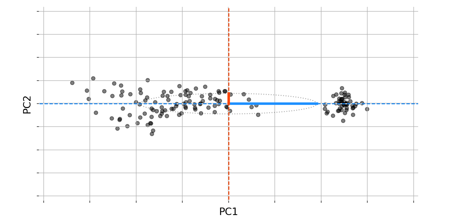
Again, we should stop and question things. Why do we care about this change of basis? Figure $3$ has the answer. Recall that our task as naturalists on a strange island is to classify all the new birds. Imagine that, being short on time, we were able to collect only beak size and wing span for the island’s birds, so we must classify them using only these two features. What Figure $3$ suggests is that in fact, we only need one feature to classify the birds: the first principal component. The fact that we do not need both features, we only need one, is a deep idea. You may know that PCA is used for dimension reduction, and this is why. PCA allows us to find new composite features based on how much variation they explain, so we can keep only those that explain a large fraction of the variance in our data. These new composite features are important, so let us name them; we will call them latent features or latent variables.

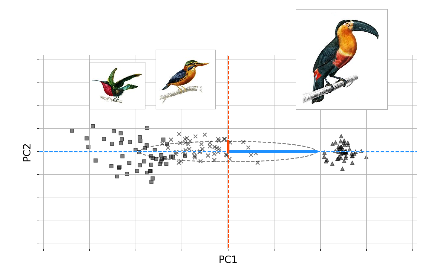
Imagine that a brillant ornithology visted our island, and correctly classified all the birds into three groups (Figure $4$). Since the first PC captures most of the variation, this would immediately suggest that if we actually looked at the birds and their groupingsAgain, we should stop and question things. Why do we care about this change of basis? Figure $3$ has the answer. Recall that our task as naturalists on a strange island is to classify all the new birds. Imagine that, being short on time, we were able to collect only beak size and wing span for the island’s birds, so we must classify them using only these two features. What Figure $3$ suggests is that in fact, we only need one feature to classify the birds: the first principal component. The fact that we do not need both features, we only need one, is a deep idea. You may know that PCA is used for dimension reduction, and this is why. PCA allows us to find new composite features based on how much variation they explain, so we can keep only those that explain a large fraction of the variance in our data. These new composite features are important, so let us name them; we will call them latent features or latent variables.

It is worth reminding ourselves that, while all this talk of “principal components,” “change of basis,” and “orthogonality” is abstract, its meaning can be interpretable and even intuitive. Imagine that a brilliant ornithologist visited our island, and correctly classified all the birds into three groups (Figure $4$). Since the first PC captures most of the variation, this suggests that if we actually looked at the birds and their groupings, we would find large beaks and large wingspans on one end of the spectrum, and small beaks and small wingspans on the other. The first PC is simply capturing the variation in both, which is possible precisely because these two features covary.

2. Formalising the objective function

Now that we understand the big picture, we can ask: how do we find these principal components? Let us turn our geometric picture into an optimisation problem.

Computing the principal components

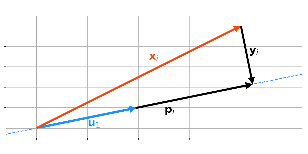
Assume our data is mean-centered, and consider an arbitrary unit vector $\mathbf{u}_1$ (Figure 5). We want to maxmise the variance of our data after it is projected onto a new axis defined by $\mathbf{u}_1$. In other words, we want to maximise the squared distance of our projected data from the origin.

To formalise this, consider an arbitrary datum in our collection, $\mathbf{x}_i$, and let’s denote the project of $\mathbf{x}_i$ onto $\mathbf{u}_1$ as $\mathbf{p}_i$:

We want to find the optimal $\mathbf{u}_1^\star$ such that the squared length of $\mathbf{p}_i$ is maximised, where the length is

This suggests the following optimisation problem:

This is the linear-algebraic formulation of the idea in the previous section: the first PC corresponds to the axis along which the variance of our projected data is maximised.

A little algebraic manipulation of the summation in Equation $3$ gives us

Equation $4$ allows us to rewrite Equation $3$ as

So the optimisation problem for finding the first PC is to optimise with respect to our data’s (mean-centered) covariance matrix. This is because we are ultimately maximising the variance of our data with respect to $\mathbf{u}_1$, and the covariance matrix captures the necessary relationships.

However, what we are about to show is even better: the first PC is actually just the first eigenvector of the covariance matrix, $\mathbf{X}^\top\mathbf{X}$. This is not an obvious result. It is surprising and beautiful. To see this, observe that since $\mathbf{X}^\top\mathbf{X}$ is a symmetric, positive-semidefinite matrix, it has an eigendecomposition.

where $\mathbf{x}$ is a square matrix $\left(P\times P\right)$ with eigenvectors for columns and where $\Lambda$ is a diagonal matrix of eigenvelues. If we define a new variable $\mathbf{w}_1$ as

then we can rewrite the optimisation problem in Equation $5$ as

The norm of $\mathbf{w}_1$ must also be unity since

Equation $9$ relies on the fact that $\mathbf{Q}$ is orthnormal and thus $\mathbf{Q}^\top\mathbf{Q}=\mathbf{Q}\mathbf{Q}^\top=\mathbf{I}_P$. Since $\lambda$ is diagonal, the bracketed term in Equation $8$ can be un-packed back into summation, giving us

where $\lambda_i$ is the $i$-th eigenvalue associated with the $i$-th column $\mathbf{Q}$. Without loss of generality, assume that the eigenvalues are ordered, $\lambda_1\leq\lambda_2\leq\cdots\leq\lambda_p\leq 0$. (Recall that these eigenvalues are all non-negative, since covariance matrices are always symmetric and positive semi-definite.) Since the eigenvalues are all non-negative, clearly the weights that maximise the problem are

In other words, the optimal $\mathbf{w}_1^\star$ is just the first standard basis vector $\mathbf{e}_1$. If we plug this optimal weight back into Equation $7$, we see that the optimal $\mathbf{w}_1$ is simply the first eigenvector

To summarise, we wanted to find the first principal component of our data. As we saw in the first section, this first principal component is a vector that defines an axis along which the variance of our projected data is maximised. Moreover, the first principal component is, in fact, the first eigenvector of our data’s covariance matrix.

Finding the second principal follows the same reasoning as above, except now we need to add a constraint: $\mathbf{u}_2$ must be orthogonal to $\mathbf{u}_1$. Intuitively, it is pretty clear that $\mathbf{w}_2^\star$ for $\mathbf{w}_2=\mathbf{Q}^\top \mathbf{u}_2$ will be second standard basis vector, $\mathbf{e}_2$, since that will “select” the second largest eigenvalue, $\lambda_2$, while ensuring that the two principal components are orthogonal, since

Of course, this is not a proof, which would probably use induction, but it captures the main idea nicely.

At this point, we may be wondering: have we just “punted” understanding principal components to understanding eigenvectors? Not necessarily. A deeper understanding of eigenvectors would be useful here. However, it is fine to say that this idea — that the eigenvectors of a covariance matrix define orthogonal axes along which our data has maximal variance — is simply one of many reasons why eigenvectors are such well-studied mathematical objects.

Maximizing variation versus minimizing error

So far, we have discussed PCA as finding a linear projection of our data such that the projected data has maximum variance. Visually, this is just finding the blue-dashed line in Figure $2$ so we can transform our data into Figure $3$. However, there is an alternative view of PCA’s objective function: it finds an axis such that the squared error between our data and the transformed data is minimised.

This connection may sound more complicated than it is. It is really just the claim that if we want to maximise the leg (not hypotenuse) of a right triangle ($\mathbf{p}_i$ in Figure $5$), we must minimise the other leg ($\mathbf{y}_i$ in Figure $5$). This StackExchange answer also includes some additional visualisations, but, in my opinion, they are essentially more complex versions of Figure $5$.

To see this formally, let us define the difference between $\mathbf{u}$ and $\mathbf{x}_i$ as $\mathbf{y}_i$. If we minimise the length of $\mathbf{y}_i$, we minimise the difference between our datum $\mathbf{x}_i$ and our projected datum $\mathbf{p}_i$. So we want to find the optimal $\mathbf{u}_i^\star$ such that the length of $\mathbf{y}_i$ is minimised:

We can write the unconstrained objective in terms of $\mathbf{u}_1$ as

Step $\star$ holds because $\mathbf{u}_1^\top \mathbf{u}_1$ and $\mathbf{x}_i^\top \mathbf{x}_i$ are constants. To minimise a negative quantity, we want to maximise the un-negated quantity. So we can write this objective as

However, this is equivalent to optimising the absolute length of $\mathbf{p}_i$, which in turn is equivalent to optimising the squared length of $\mathbf{p}_i$.

It is useful to understand this connection, but the real intuition is Figure $5$. PCA finds principal components $\mathbf{u}_1,\ldots,\mathbf{u}_P$ such that the variance of our projected data is maximised, which is equivalent to the squared error of our projected data being maximised (with respect to the original data).

Deriving basic properties

Let’s start by computing principal components. Let $\mathbf{X}$ be an $N\times P$ mean-centered designed matrix of our data. The $P$ columns are features, while the $N$ rows are independent samples. We saw in the previous section that the principal components are just eigenvalues of the covariance matrix of $\mathbf{X}$. The empirical covariance matrix of our data is

So $\mathbf{C}_X$ is a $P\times P$ symmetric and positive semi-definite matrix. The eigendecomposition of $\mathbf{C}_X$ is

where $\Lambda$ is a diagonal matrix of eigenvalues, and where $\mathbf{Q}$ is a $P\times P$ matrix whose columns are eigenvectors, i.e. principal components. In other words, the columns of $\mathbf{Q}$ are unit vectors that point in orthogonal directions of maximal variation (e.g. the red and blue arrows in Figure $2$).

Note that we can also compute the principal component via the SVD. The SVD of $\mathbf{X}$ is

where $\mathbf{U}$ is unitary and $N\times P,\mathbf{S}$ is diagonal and $P\times P$, and $\mathbf{V}$ is unitary and $P\time P$. We can write our empirical covariance matrix $\mathbf{C}_X$ via this SVD:

Here, $\mathbf{S}^2$ denotes a diagonal matrix with the squared singular values of $\mathbf{S}$. Thus, we can use the SVD to diagonalise our matrix $\mathbf{C}_X$. This immediately suggests a relationship between singular values and eigenvalues, namely:

Note that since $\mathbf{C}_X$ is symmetric and positive semi-definite, its eigenvalues are non-negative. Thus, the singular values and the eigenvalues tell the same story: they scale the variation for their respective principal components.

Transformed data

Now that we know how to compute the principal components $\mathbf{V}$, let’s use them to transform our data (e.g. from Figures $2$ to $3$)

The matrix $\mathbf{V}$ perform a change of basis on $P$-vectors such that after the linear transformation, the standard basis vectors are mapped to the columns (eigenvectors) of $\mathbf{V}$. Visually, $\mathbf{V}$ un-whitens vectors by rotating them from Figure $3$ back into Figure $2$. Let $\mathbf{z}_i$ be a vector in this whitened vector space. Then we can represent a single datum $\mathbf{x}_i$ (also a $P$-dimensional column vector) as

So $\mathbf{x}_i$ is our un-whitened data. Since $\mathbf{x}_i$ is a column vector here but a row vector in $\mathbf{X}$, we can represent Equation $22$ as a matrix operation as

We can write this transformation via the SVD as

This linear transformation, $\mathbf{XV}$, transforms our data $\mathbf{X}$ into latent variables $\mathbf{Z}$.

When we use PCA for dimension reduction, then $\mathbf{V}$ has shape $P\times K$ and $\mathbf{S}$ has shape $P$, where $K$ is the number of reduced features and where ideally $K\ll P$. In this framing, we can view $\mathbf{ZV}^\top$ as a low-rank approximation of $\mathbf{X}$. So an alternative view of PCA is that we are finding a low-rank approximation of our data matrix, capturing its basic structure with fewer parameters.

Note that an alternative proof of the equivalence between maximising variation and minimising error is to work with the squared error $\lVert \mathbf{X}-\mathbf{XV} \rVert_2^2$.

Latent variables with uncorrelated features

We claimed that after transforming our data $\mathbf{X}$ with the principal components $\mathbf{V}$, our latent data $\mathbf{Z}$ has features with zero correlation. Let’s prove this. The covariance matrix of $\mathbf{Z}$ is:

Clear, $\mathbf{C}_Z$ is a diagonal matrix, meaning $\mathbf{Z}$ has uncorrelated features. Furthermore, we can see that the variances of our transformed data’s features are simply the eigenvalues of the covariance matrix of $\mathbf{X}$. So the standard deviations in Figure $3$ (the length of the principal components) are just the square roots of the eigenvalues.

Dimension reduction and variance explained

Now that we can compute the variances of the features of $\mathbf{Z}$, we can answer an important question: how many principal components should we use when performing dimension reduction with PCA? Answer: We take only the principal components with the largest eigenvalues, since those correspond to the largest variances.

In particular, we use the ratio of explained variance to total variance. The explained variance of a given principal component is just the variance of its associated feature (column in \mathbf{Z}), while the total variance is the sum of these explained variances. If we divide the former by the latter, we get a set of ratios that sum to unity and represent the fraction of variances explained by each feature.

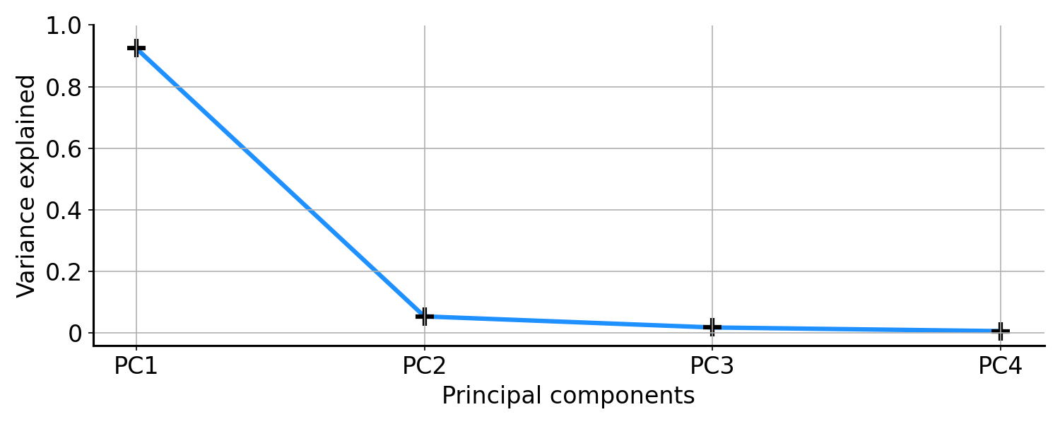
A common approach to visualising all this is a scree plot. In a scree plot, we plot the sorted principal components against the ratio of explained variances (e.g. Figure $6$). Ideally, we would want our scree plot to look like a hockey stick. The elbow of the stick is where the eigenvalues level off. We would only want to take the components with large eigenvalues, since they explain most of the variation in our data. For example, in Figure $3$ it is clear that the first principal component has much larger eigenvalue than the second. So if we could only pick one component, we would pick the first one.

Unchanged total variance

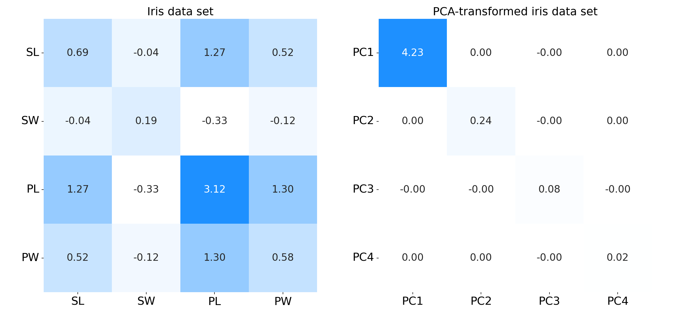
An interesting and intuitive property of PCA is that total variance of our raw data is identical to the total variance of our transformed data. Concretely, the sum of the diagonals of their respective covariance matrices are the same. For example, consider the two covariance matrices in Figure $7$. The left subplot is the covariance matrix of some clearly correlated data $\mathbf{X}$, while the right subplot is the covariance matrix of our transformed data $\mathbf{Z}$. You can check for yourself that the sum of the diagonals are identical (roughly $4.57$).

To see this formally, let’s compute the total variance of both our data $\mathbf{X}$ and the transformed data and $\mathbf{Z}$. Clearly, the total variance of $\mathbf{Z}$ is just the sum of the diagonal (eigenvalues) in $\mathbf{C}_Z$, since it is diagonal matrix:

However, the total variance of $\mathbf{X}$ is trickier, since $\mathbf{C}_X$ is not a diagonal matrix. We want to prove that the sum of the diagonals of $\mathbf{C}_X=\mathbf{Q}\Lambda \mathbf{Q}^\top$ is equal to the sum of the eigenvalues. Intuitively, we might suspect this is true since $\mathbf{Q}$ is a unitary matrix.

First, let’s write out the terms of $\mathbf{Q}$ explicity:

Then $\Lambda \mathbf{Q}^\top$

and $\mathbf{W}\Lambda \mathbf{Q}^\top$

Writing out each term in this product matrix would be tedious, but it is clear that the $i$-th diagonal element in this matrix is

and so the sum of the diagonals must be

We can group all the terms associated with the same $\lambda_i$. This gives us

and each inner summation is really the squared norm of a row of $\mathbf{Q}$. Since $\mathbf{Q}$ is unitary, these squared norms are unity. So the sum of the diagonal elements of $\mathbf{C}_X$ is the sum of the eigenvalues. To summarise this subsection, we have shown:

This is fairly intuitive. For any given data set, there is some total variation. If we apply some linear transformation to our data, we change how the features are correlated, but we don’t change the total variation inherent in the data.

Loadings

In PCA, we decompose the covariance matrix into directions (PCs) and scales (eigenvalues). However, we often want to combine these two bits of information into scaled vectors (e.g., the solid axes lines in Figure $2$). In the language of PCA and factor analysis, the loadings are the principal components scaled by the square roots of the respective eigenvalues. In other words, loadings are scaled by the standard deviations of the transformed features. Concretely, let $\mathbf{L}$ be a $P\times P$ matrix of factor loadings. Then

Conversely, eigenvectors are unit-scaled loadings.

Probabilitic PCA

We can frame PCA as a probabilistic model, called probabilistic PCA (Tipping & Bishop, 1999). The statistical model for probabilistic PCA is

Why is this the correct probabilistic framing? Tripping & Bishop have a deeper analysis, but here is one way to think about it. One view of PCA is that we decompose (or approximate) our design matrix $\mathbf{X}$ via a linear transformation of latent variables $\mathbf{Z}$:

And the covariance matrix of $\mathbf{X}$ is proportional to

We can see that Equation $35$ models the same relationships, since it implies that $\mathbf{x}_i$ is normally distributed as

So the model in Equation $35$ is analogous to the model we have discussed so far.

Exploring a complete example

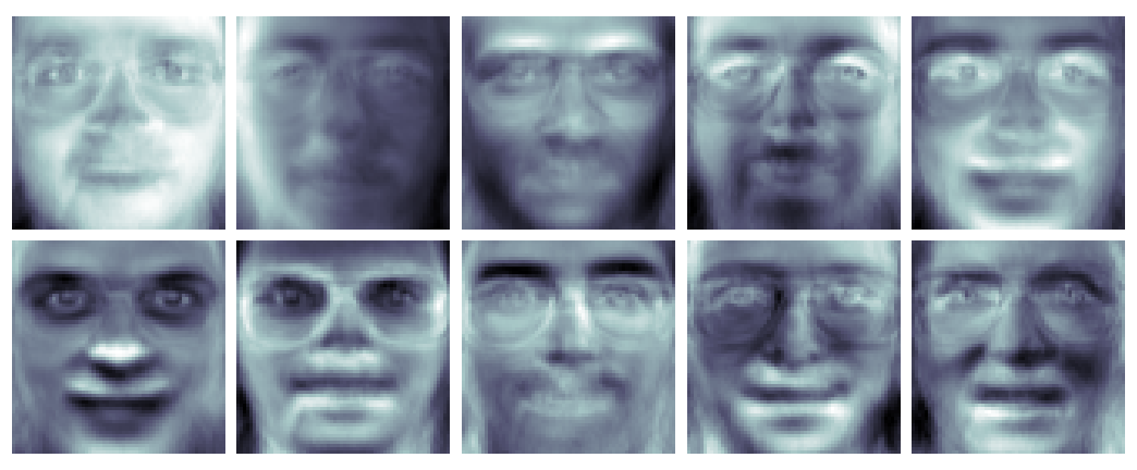
As an example of the power of PCA, let us reproduce a famous result, eigenfaces (Turk & Pentland, 1991). An eigenface is simply a principal component of a data set of face images. Since principal components form a basis for the images in our data set, visualising a single eigenface yields an eerie, idealised face. See Figure $8$ for eigenfaces based on the Olivetti face database.

What does the definition of eigenfaces really mean? Recall Equation $22$, which we will rewrite here:

If $\mathbf{x}_i$ is a $P$-vector representing an image with $P$ pixels and if an eigenface is a column of $\mathbf{V}$, then $\mathbf{z}_i$ must be a $P$-vector representing how much each eigenfaces (out of $P$ eigenfaces) contributes to $\mathbf{x}_i$. It may be helpful to write out the matrix-multiplication in Equation $39$ more diagrammatically:

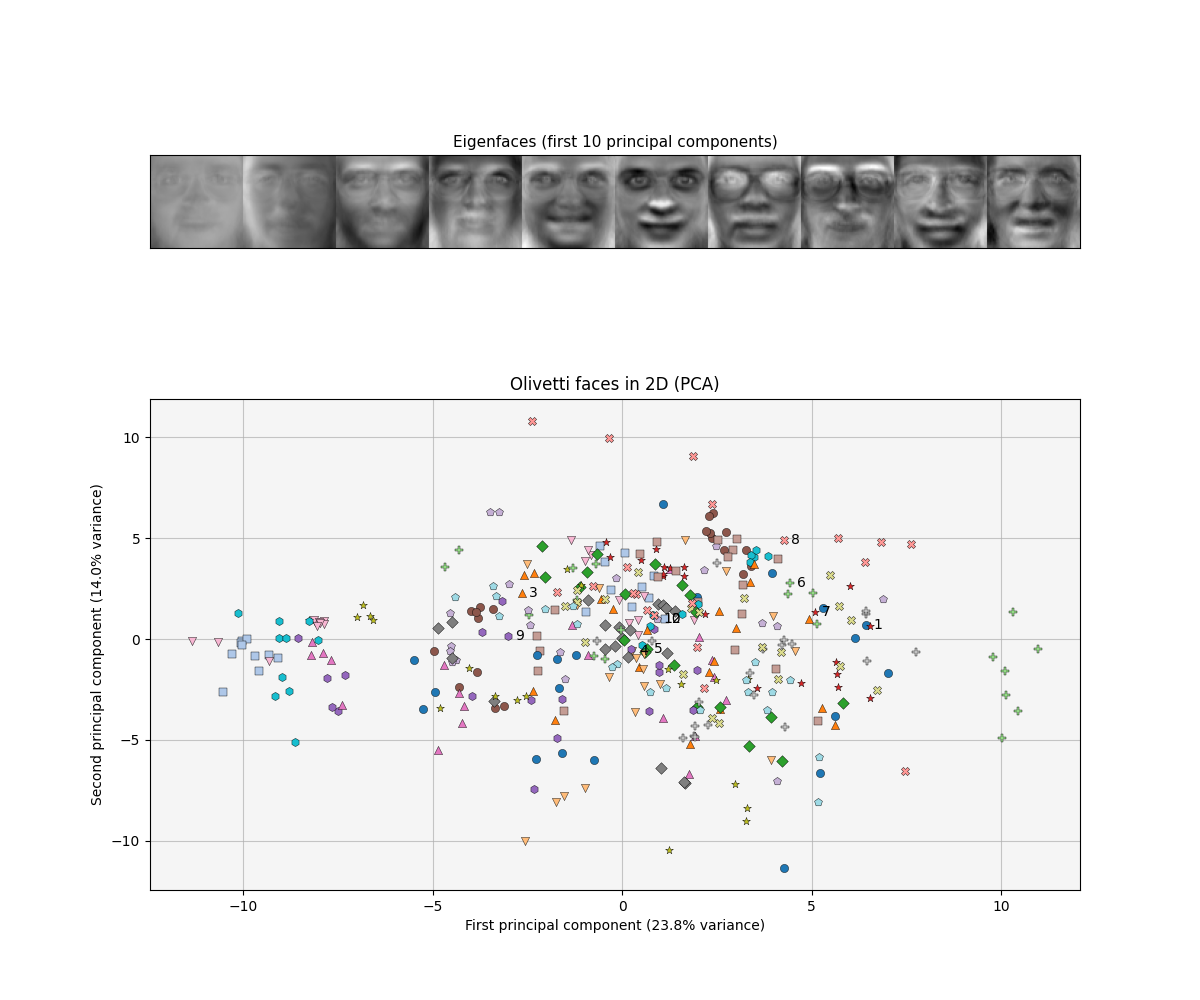
So each datum (the image on the left-hand side of Equation $40$) is a linear combination of eigenfaces, with coefficients defined by the latent variable. However, what is the utility of an eigenface? If we can find a small set of eigenfaces–say $K$ where $K \ll P$ pixels–then we can find a lower-dimensional representation of our data that can be used for downstream tasks like visualisation, data compression, and classification. For example, we could sort out eigenfaces by their associated eigenvalues and only pick the top two eigenfaces. Moreover, two could visualise the two latent pixels for each image (Figure $9$).

While eigenfaces are abstract, recall that this is precisely what we were trying to do when we imagined ourselves as naturalists classifying birds on a strange island. We have abstracted the problem further, where instead of collecting beaks and feathers, we collect pixels. On the island, we were able to construct a composite feature “bird size” from “beak size” and “wing span” because the two features were correlated. With eigenfaces, we can construct composite images or project pixels because many pixels in our data are correlated.

Code for implementing the PCA is provided here.

Conclusion

Principal components are a collection of orthogonal unit vectors such that the $i$-th principal component captures maximum variation in our data, while being orthogonal to the previous $i-1$ PCs. Thus, principal components provide a basis for transforming our data into latent variables. These latent variables capture correlations among our data’s features, allowing for a reduced set that roughly captures the same amount of total variation.

Given today’s advances in computer vision, the eigenface results may not be particularly impressive. For example, one could easily fit an autoencoder to produce much higher-quality latent variables for clustering. However, this is the wrong perspective. In context, it should be surprising that a simple linear model, such as PCA, is so effective on high-dimensional, richly structured data like images. Given that it is also fast, easy to implement, and well understood theoretically, PCA is a great first choice for preliminary data analysis.

References

1. Pearson, K. (1901). On lines and planes of closest fit to systems of points in space. The London, Edinburgh, and Dublin Philosophical Magazine and Journal of Science, 2(11), 559-572.
2. Hotelling, H. (1933). Analysis of a complex of statistical variables into principal components. Journal of Educational Psychology, 24(6), 417.
3. Turk, M., & Pentland, A. (1991). Eigenfaces for recognition. Journal of Cognitive Neuroscience, 3(1), 71-86.
4. Tipping, M. E., & Bishop, C. M. (1999). Probabilistic principal component analysis. Journal of the Royal Statistical Society: Series B (Statistical Methodology), 61(3), 611-622.