High-Dimensional Variance
December 28, 2025
When $X$ is a scalar random variable, its variance, denoted $\mathbb{V}[X]$, is defined as the expected squared deviation from its mean:
\[\begin{equation} \mathbb{V}[X]:=\sigma^2=\mathbb{E}\left[(X-\mathbb{E}[X])^2\right] \end{equation}\]The mean $\mathbb{E}[X]$ characterises the central tendency of $X$, whereas the variance $\mathbb{V}[X]$ quantifies the degree to which realisations of $X$ are dispersed around that centre. Both quantities are moments of the underlying distribution.
When $\mathbf{X}$ is instead a random vector—that is, an ordered collection of scalar random variables,
\[\begin{equation} X=\begin{bmatrix} X_1\\ X_2\\ \vdots\\ X_n \end{bmatrix}, \end{equation}\]it is less common, at least in standard terminology, to refer directly to the variance of $\mathbf{X}$. Rather, one typically speaks of the covariance matrix of $\mathbf{X}$, denoted $\text{cov}(\mathbf{X})$:
\[\begin{equation} \text{cov}(\mathbf{X}):=\Sigma=\mathbb{E}\left[(\mathbf{X}-\mathbb{E}[\mathbf{X}])(\mathbf{X}-\mathbb{E}[\mathbf{X}])^\top\right]. \end{equation}\]Equations $1$ and $3$ are evidently similar in form. This raises a natural question: should the covariance matrix be understood as a higher-dimensional, or multivariate, analogue of variance? In other words, is it meaningful to write
\[\begin{equation} \mathbb{V}[\mathbf{X}]:=\text{cov}[\mathbf{X}] \end{equation}\]and interpret this object as the variance of a random vector?
This interpretation is certainly not novel, nor was it the way in which covariance matrices were first introduced to me. Nevertheless, it provides a useful conceptual bridge between the scalar and multivariate cases. The purpose of this note is therefore to examine the extent to which a covariance matrix may be regarded as a high-dimensional generalisation of variance.
Definitions
The relationship between variance and covariance is already apparent from their definitions. Expanding the outer product in Equation $3$ gives
\[\begin{equation} \Sigma=\begin{bmatrix} \mathbb{E}[(X_1-\mathbb{E}[X_1])^2] & \ldots & \mathbb{E}[(X_1-\mathbb{E}[X_1])(X_n-\mathbb{E}[X_n])]\\ \vdots & \ddots & \vdots\\ \mathbb{E}[(X_n-\mathbb{E}[X_n])(X_1-\mathbb{E}[X_1])] & \ldots& \mathbb{E}[(X_n-\mathbb{E}[X_n])^2]\\ \end{bmatrix}, \end{equation}\]The diagonal entries of $\Sigma$ are precisely the variances of the scalar components $X_i$. Thus, $\text{cov}[\mathbf{X}]$ continues to encode the marginal dispersion of each coordinate of the random vector.
The off-diagonal entries, by contrast, describe pairwise covariation. For variables $X_i$ and $X_j$, the corresponding covariance is defined as
\[\begin{equation} \sigma_{ij}:=\text{cov}\left(X_i, X_j\right)=\mathbb{E}\left[(X_i-\mathbb{E}[X_i])(X_j-\mathbb{E}[X_j])\right]. \end{equation}\]Equation $6$ generalises Equation $1$, with ordinary variance recovered as the special case $i = j$:
\[\begin{equation} \mathbb{V}[X_i]=\text{cov}(X_i, X_i). \end{equation}\]The quantity $\sigma_{ij}$ depends not only on the marginal variances of $X_i$ and $X_j$, but also on the degree to which the two variables vary together. For instance, even if $X_i$ and $X_j$ each have large variance, their covariance may be small if they are statistically uncorrelated: large or small realisations of one variable do not systematically correspond to large or small realisations of the other. This behaviour is illustrated in Figure $1$.
This observation motivates the familiar expression of covariance in terms of the Pearson correlation coefficient $\rho_{ij}$:
\[\begin{equation} \sigma_{ij}=\rho_{ij}\sigma_{i}\sigma_{j} \end{equation}\]This formula also extends the variance case, since $\rho_{ij}=1$ whenever $i=j$.
Using the notation in Equation $8$, the covariance matrix can be written as
\[\begin{equation} \Sigma= \begin{bmatrix} \sigma_1^2 & \rho_{12}\sigma_1\sigma_2 & \cdots & \rho_{1n}\sigma_1\sigma_n \\ \rho_{21}\sigma_2\sigma_1 & \sigma_2^2 & \cdots & \rho_{2n}\sigma_2\sigma_n \\ \vdots & \ddots & \cdots & \vdots \\ \rho_{n1}\sigma_n\sigma_1 & \rho_{n2}\sigma_n\sigma_2 & \cdots & \sigma_n^2\\ \end{bmatrix}. \end{equation}\]A straightforward algebraic rearrangement yields the decomposition
\[\begin{equation} \Sigma= \begin{bmatrix} \sigma_1 &&&\\ &\sigma_2 &&\\ &&\ddots& \\ &&& \sigma_n \\ \end{bmatrix} \begin{bmatrix} 1 & \rho_{12} & \ldots & \rho_{1n}\\ \rho_{21} & 1 & \ldots & \rho_{2n}\\ \ldots & \ldots & \ddots & \ldots\\ \rho_{n1} & \rho_{n2} & \ldots & 1\\ \end{bmatrix} \begin{bmatrix} \sigma_1 &&&\\ &\sigma_2 &&\\ &&\ddots& \\ &&& \sigma_n \\ \end{bmatrix}. \end{equation}\]The middle matrix is the correlation matrix, which records the Pearson linear correlations between all pairs of variables in $\mathbf{X}$. Consequently, the covariance matrix simultaneously represents the marginal variances of the components $X_i$ and the pairwise covariances among them. If scalar variance is viewed as a one-dimensional covariance matrix, then the univariate case can be expressed as
\[\begin{equation} \Sigma=[\text{cov}(X,X)]=[\sigma][1][\sigma]. \end{equation}\]Although Equation $11$ has little practical importance, it makes explicit that ordinary variance is a special case of the covariance matrix.
Equation $10$ also gives a direct way to obtain the correlation matrix $\mathbf{C}$ from the covariance matrix $\Sigma$:
\[\begin{equation} \mathbf{C}:= \begin{bmatrix} 1/\sigma_1 & & \\ &\ddots& \\ & & 1/\sigma_n \\ \end{bmatrix} \Sigma \begin{bmatrix} 1/\sigma_1 & & \\ &\ddots& \\ & & 1/\sigma_n \\ \end{bmatrix} \end{equation}\]This follows from the fact that the inverse of a diagonal matrix is obtained by taking the reciprocal of each diagonal entry.
Properties
Several fundamental properties of scalar variance have natural multivariate analogues. For example, if $a$ is a deterministic scalar, then the variance of $aX$ scales quadratically:
\[\begin{equation} \mathbb{V}[aX]=a^2\mathbb{V}[X]=a^2\sigma^2. \end{equation}\]In the multivariate setting, if $\mathbf{A}$ is a deterministic matrix, then
\[\begin{equation} \begin{aligned} \mathbb{V}[\mathbf{A}\mathbf{X}]&=\mathbf{A}\Sigma\mathbf{A}^\top \\ &=\mathbb{E}\left[(\mathbf{A}\mathbf{X}-\mathbb{E}[\mathbf{A}\mathbf{X}])(\mathbf{A}\mathbf{X}-\mathbb{E}[\mathbf{A}\mathbf{X}])^\top\right]\\ &=\mathbf{A}\mathbb{E}\left[(\mathbf{X}-\mathbb{E}[\mathbf{X}])(\mathbf{X}-\mathbb{E}[\mathbf{X}])^\top\right]\mathbf{A}^\top \\ &=\mathbf{A}\Sigma\mathbf{A}^\top \end{aligned} \end{equation}\]Thus, both scalar variance and covariance matrices transform quadratically under multiplicative linear transformations.
Similarly, scalar variance is invariant under translation. For a deterministic scalar $a$,
\[\begin{equation} \mathbb{V}[a+X]=\mathbb{V}[X]. \end{equation}\]Adding a constant shifts the location of a distribution but does not alter its spread. The same principle holds in multiple dimensions: adding a deterministic vector leaves the covariance matrix unchanged.
\[\begin{equation} \begin{aligned} \mathbb{V}[\mathbf{A}+\mathbf{X}]&=\mathbb{E}\left[(\mathbf{A}+\mathbf{X}-\mathbb{E}[\mathbf{A}+\mathbf{X}])(\mathbf{A}+\mathbf{X}-\mathbb{E}[\mathbf{A}+\mathbf{X}])^\top\right]\\ &=\mathbb{E}\left[(\mathbf{X}-\mathbb{E}[\mathbf{X}])(\mathbf{X}-\mathbb{E}[\mathbf{X}])^\top\right]\\ &=\Sigma \end{aligned} \end{equation}\]Variance also admits the well-known decomposition
\[\begin{equation} \mathbb{V}[X]=\mathbb{E}\left[X^2\right]-\mathbb{E}[X]^2 \end{equation}\]The vector-valued analogue is
\[\begin{equation} \begin{aligned} \mathbb{V}[\mathbf{X}]&=\mathbb{E}\left[(\mathbf{X}-\mathbb{E}[\mathbf{X}])(\mathbf{X}-\mathbb{E}[\mathbf{X}])^\top\right]\\ &=\mathbb{E}\left[\mathbf{X}\mathbf{X}^\top-2\mathbb{E}[\mathbf{X}]\mathbf{X}^\top+\mathbb{E}[\mathbf{X}]\mathbb{E}[\mathbf{X}]^\top \right]\\ &=\mathbb{E}\left[\mathbf{X}\mathbf{X}^\top\right]-\mathbb{E}[\mathbf{X}]\mathbb{E}[\mathbf{X}]^\top \end{aligned} \end{equation}\]The purpose of these examples is not to provide an exhaustive catalogue of covariance identities, but to emphasise that many familiar properties of variance persist in higher dimensions.
Non-negativity
Another important parallel is non-negativity. In the scalar case, variance is always non-negative:
\[\begin{equation} \mathbb{V}[X]=\sigma^2\geq 0. \end{equation}\]The corresponding multivariate statement is that covariance matrices are positive semi-definite (PSD):
\[\begin{equation} \mathbb{V}[X]=\Sigma\geq 0, \end{equation}\]In this sense, positive semi-definiteness is the matrix-valued analogue of non-negativity.
The Cholesky decomposition of a PSD matrix may therefore be interpreted as a natural extension of the scalar square root. The Cholesky factor $\mathbf{L}$ plays a role analogous to a multivariate standard deviation, since
\[\begin{equation} \Sigma=\mathbf{L}\mathbf{L}^\top\implies\mathbf{L}\approx\sigma \end{equation}\]Here, the symbol ‘$\approx$’ is intended only as an analogy, not as a literal equality.
Precision and whitening
For a scalar random variable, precision is defined as the reciprocal of variance:
\[\begin{equation} p=\frac{1}{\sigma^2} \end{equation}\]Higher precision corresponds to lower variance and therefore to less dispersion in possible outcomes. This notion appears naturally in standardisation, or whitening, where data are transformed to have zero mean and unit variance. In the scalar case, this is achieved by subtracting the mean and dividing by the standard deviation:
\[\begin{equation} Z=\frac{X-\mathbb{E}[X]}{\sigma} \end{equation}\]This transformation is often called z-scoring.
The multivariate analogue is obtained through the precision matrix $\mathbf{P}$, defined as the inverse of the covariance matrix:
\[\begin{equation} \mathbf{P}=\Sigma^{-1}. \end{equation}\]Given the Cholesky decomposition in Equation $21$, the precision matrix can be written as
\[\begin{equation} \begin{aligned} \mathbf{P}&=\left(\mathbf{L}\mathbf{L}^{\top}\right)^{-1}\\ &=\left(\mathbf{L}^{\top}\right)^{-1}\mathbf{L}^{-1}\\ &=\left(\mathbf{L}^{-1}\right)^{\top}\mathbf{L}^{-1}\\ \end{aligned} \end{equation}\]Thus, the multivariate counterpart of the z-score is
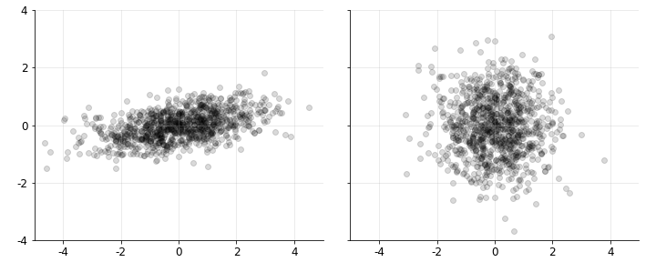
\[\begin{equation} \mathbf{Z}=\mathbf{L}^{-1}(\mathbf{X}-\mathbb{E}[\mathbf{X}]). \end{equation}\]Geometrically, this transformation linearly maps samples from a random vector with covariance $\Sigma$ into a new coordinate system in which the resulting variables have identity covariance. This whitening effect is shown in Figure $2$.
Ignoring the mean for simplicity, this claim can be verified directly:
\[\begin{equation} \begin{aligned} \mathbb{V}[Z]&=\mathbb{E}\left[\left(\mathbf{L}^{-1}\mathbf{X}\right)\left(\mathbf{L}^{-1}\mathbf{X}\right)^\top\right]\\ &=\mathbb{E}\left[\mathbf{L}^{-1}\mathbf{X}\mathbf{X}^\top\left(\mathbf{L}^{-1}\right)^\top\right]\\ &=\mathbf{L}^{-1}\mathbb{E}\left[\mathbf{X}\mathbf{X}^\top\right]\left(\mathbf{L}^{-1}\right)^\top\\ &=\mathbf{L}^{-1}\Sigma\left(\mathbf{L}^\top\right)^{-1}\\ &=\mathbf{I}\\ \end{aligned} \end{equation}\]Including the mean slightly lengthens the derivation, but it does not alter the underlying argument. A full discussion of why the Cholesky decomposition produces this transformation would require a separate treatment; related geometric ideas also appear in principal component analysis (PCA).
Summary statistics
It is often useful to summarise the information contained in a covariance matrix using a single scalar quantity. Two common summaries are total variance and generalised variance, each of which captures a different aspect of the covariance structure.
Total variance. The total variance of a random vector $\mathbf{X}$ is defined as the trace of its covariance matrix:
\[\begin{equation} \sigma*{\text{tv}}^2:=\text{tr}(\Sigma)=\sum*{i=1}^n\sigma\_{i}^2. \end{equation}\]This quantity aggregates the marginal variances across all components of $\mathbf{X}$. It is especially important in PCA, where total variance is preserved under orthogonal transformations. In one dimension, total variance reduces to ordinary variance: $\sigma_{\text{tv}}^2=\sigma^2$.
Generalised variance. The generalised variance (Wilks, 1932) of a random vector $\mathbf{X}$ is defined as the determinant of its covariance matrix:
\[\begin{equation} \sigma\_{\text{gv}}^2:=\text{det}(\Sigma)=|\Sigma|. \end{equation}\]The determinant has rich geometric interpretations, but in this context it is useful to view it as the product of the eigenvalues of $\Sigma$:
\[\begin{equation} |\Sigma|=\prod\_{i=1}^n\lambda_i. \end{equation}\]Thus, the generalised variance reflects the overall scale of the linear transformation represented by $\Sigma$.
Generalised variance and total variance can behave quite differently. For example, consider a two-dimensional covariance matrix satisfying
\[\begin{equation} \sigma_1=\sigma_2=\rho=1 \end{equation}\]In this case, the total variance is two, whereas the determinant is one. If the variables are instead highly correlated, for instance with $\rho=0.98$, the total variance remains two, but the determinant falls to approximately $0.039$, indicating near-singularity. Total variance therefore measures aggregate marginal spread, whereas generalised variance is sensitive to the dependence structure among the components of $\mathbf{X}$. Strong correlations can substantially reduce the effective volume described by the covariance matrix.
Example
We conclude with two examples that illustrate the preceding ideas.
Multivariate normal. First, recall the probability density function (PDF) of a univariate normal random variable:
\[\begin{equation} p\left(x;\mu,\sigma^2\right)=\frac{1}{\sqrt{2\pi}\sigma}\exp\left\lbrace -\frac{1}{2}\left(\frac{x-\mu}{\sigma}\right)^2 \right\rbrace. \end{equation}\]The squared term in the exponent is precisely the square of the standardised quantity from Equation $23$. If the covariance matrix is interpreted as a higher-dimensional variance, then the corresponding density for a multivariate normal random variable is
\[\begin{equation} p\left(\mathbf{x};\mu,\Sigma \right)=\frac{1}{(2\pi)^{-n/2}|\Sigma|^{-1/2}}\exp\left\lbrace -\frac{1}{2}(\mathbf{x}-\mu)^{\top}\Sigma^{-1}(\mathbf{x}-\mu) \right\rbrace. \end{equation}\]Here, the Mahalanobis distance plays a role analogous to the squared z-score in the univariate case. Likewise, the univariate normalising factor
\[\begin{equation} \frac{1}{\sqrt{2\pi}\sigma} \end{equation}\]is replaced by a multivariate normalising term involving the generalised variance.
Correlated random variables. Now consider a scalar random variable $Z$ with unit variance, so that $\mathbb{V}[Z]=1$. Multiplying $Z$ by $\sigma$ gives a new random variable $X$ with variance $\sigma^2$:
\[\begin{equation} \mathbb{V}[\sigma Z]=\sigma^2\mathbb{V}[Z]=\sigma^2. \end{equation}\]The same idea extends naturally to higher dimensions. Suppose that we begin with two independent random variables,
\[\begin{equation} Z= \begin{bmatrix} Z_1 \\ Z_2 \\ \end{bmatrix}, \end{equation}\]and wish to construct a random vector $\mathbf{X}$ with a prescribed covariance matrix $\Sigma$. A standard approach is to multiply $\mathbf{Z}$ by the Cholesky factor associated with the desired covariance matrix, as in Equation $26$.
This gives a general procedure for generating correlated random variables: first generate $\mathbf{Z}$ with independent components of unit variance, and then multiply by the Cholesky factor of the target covariance matrix. In the $2\times2$ case,
\[\begin{equation} \text{cholesky}\left(\begin{bmatrix}1&\rho\\ \rho&1\\\end{bmatrix} \right)=\mathbf{L}\mathbf{L}^{\top}=\begin{bmatrix}1&0\\ \rho&\sqrt{1-\rho^2}\end{bmatrix} \begin{bmatrix}1&\rho\\ 0&\sqrt{1-\rho^2} \end{bmatrix} \end{equation}\]Thus, one may draw two independent random variables $Z_1$ and $Z_2$, each with unit variance, and define
\[\begin{equation} \begin{aligned} X_1&:=Z_1\\ X_2&:=Z_1\rho+Z_2\sqrt{1-\rho^2}\\ \end{aligned} \end{equation}\]This construction generalises directly to arbitrary dimension, and non-unit marginal variances can be incorporated by choosing the appropriate covariance matrix.
Conclusion
From this perspective, it is natural to regard $\Sigma$ as a form of variance for a random vector, written suggestively as $\mathbb{V}[\mathbf{X}]$. This interpretation helps clarify several properties of covariance matrices, including positive semi-definiteness and the role of matrix inverses in whitening transformations. At the same time, multivariate variance contains structure that has no counterpart in the scalar case, most notably the correlations and covariances among distinct components of $\mathbf{X}$. A particularly useful viewpoint, therefore, is to treat ordinary variance as the one-dimensional special case of the covariance matrix. This framing preserves the familiar intuition of variance while extending it to the richer geometry of high-dimensional random variables.